From Qiime2 into R - Initial diagnostics
Packages
library(qiime2R)
library(tidyverse)
library(stringr)
library(vegan)
library(phyloseq)
Import qiime files
## use this vector to set factor levels (this is only needed if you want treatments
## in a certain order for your figures)
### 'levelsvector' is added to steps below.
levelsvector = c("Control", "H2O2","Heat", "Inositol", "SodiumFormate", "SodiumAcetate",
"CitricAcid", "FumaricAcid",  "Lime", "PoultryLitter", "Biochar")

## metadata
# This is the same metadata file that was used in qiime2
metadata<- readr::read_tsv("metadata.tsv")
metadata2 <- metadata[c(2:nrow(metadata)),c(1:length(metadata))] %>%
  tibble::rownames_to_column("spl") %>%
  dplyr::mutate_all(type.convert) %>%
  dplyr::mutate_if(is.factor, as.character) %>%
  tibble::column_to_rownames("spl")

# rename, add or edit factors
metadata2$Treatment[metadata2$Treatment == "AutoclavedControl"] <- "Heat"
metadata2$Treatment <- factor(metadata2$Treatment, levels=levelsvector)
metadata2$Week <- factor(metadata2$Week, levels=c("T0","T39","T52","Reference", "Blank"))
metadata2 <- metadata2 %>% as_tibble() %>% column_to_rownames("#SampleID")

## Import of Qiime2 feature table (ASV abundances)
SVs <- qiime2R::read_qza("feature_table_insertiontreefiltered.qza")

## Import taxonomy file
## I found it easier to use a tsv file. I.e. after creating the qiime taxonomy.qzv I
## opened the file visualisation in https://view.qiime2.org/ and downloaded the .tsv from there.

taxonomy <- read_tsv("taxonomy_silva.tsv") %>%
  filter(Taxon != "categorical")  %>%
  rename(Feature.ID = `Feature ID`)

## re-format the taxonomy file to split the taxonomy into columns
## remove the confidence column
taxtable <- taxonomy %>% as_tibble() %>%
  separate(Taxon, sep=";", c("Kingdom","Phylum","Class","Order","Family","Genus","Species"))  %>%
  dplyr::select(-Confidence) %>%
  column_to_rownames("Feature.ID") %>%
  as.matrix()

## Import qiime tree file, here the insertion-tree.qza, see https://library.qiime2.org/plugins/q2-fragment-insertion/16/
tree <- read_qza("insertion-tree-silva.qza")
Create a phyloseq object
## combine all to a phyloseq object
physeqB <- phyloseq::phyloseq(
  phyloseq::otu_table(SVs$data, taxa_are_rows = T),
  phyloseq::phy_tree(tree$data),
  phyloseq::tax_table(taxtable),
  phyloseq::sample_data(metadata2) )

## Remove those annoying short codes in front of taxa names (i.e. p__ etc) as they
## dont look good in visualisation
tax_table(physeqB)[, "Kingdom"] <- str_replace_all(tax_table(physeqB)[, "Kingdom"], "d__", "")
tax_table(physeqB)[, "Phylum"] <- str_replace_all(tax_table(physeqB)[, "Phylum"], " p__", "")
tax_table(physeqB)[, "Class"] <- str_replace_all(tax_table(physeqB)[, "Class"], " c__", "")
tax_table(physeqB)[, "Order"] <- str_replace_all(tax_table(physeqB)[, "Order"], " o__", "")
tax_table(physeqB)[, "Family"] <- str_replace_all(tax_table(physeqB)[, "Family"], " f__", "")
tax_table(physeqB)[, "Genus"] <- str_replace_all(tax_table(physeqB)[, "Genus"], " g__", "")
tax_table(physeqB)[, "Species"] <- str_replace_all(tax_table(physeqB)[, "Species"], " s__", "")

physeqB
## phyloseq-class experiment-level object
## otu_table()   OTU Table:         [ 22271 taxa and 136 samples ]
## sample_data() Sample Data:       [ 136 samples by 6 sample variables ]
## tax_table()   Taxonomy Table:    [ 22271 taxa by 7 taxonomic ranks ]
## phy_tree()    Phylogenetic Tree: [ 22271 tips and 22189 internal nodes ]
Initial filtering
Filter out any ASVs that have less than 10 reads and are present in less than 3 samples. Then filter out any phyla that came up as uncharacterized and taxa that came up as mitochondria and chloroplast.
# filter as needed. This will be your final otu-table.
# Although you can still filter for specific analysis if needed.
# minimum of reads per feature
physeqB.flt = prune_taxa(taxa_sums(physeqB) >= 10, physeqB) #minimum reads per feature
physeqB.flt = filter_taxa(physeqB.flt, function(x) sum(x > 0) > (0.015*length(x)), TRUE) #minimum presense in x% of samples (136 * 0.015 = 2 samples)
#filter any phyla that have not been classified i.e. are "NA"
physeqB.flt = subset_taxa(physeqB.flt, !is.na(Phylum) & !Phylum %in% c("", "uncharacterized"))

# Filter out non-bacteria, mitochondia and chloroplast taxa
physeqB.flt <- physeqB.flt %>%
  subset_taxa(Kingdom == "Bacteria" & Family  != "Mitochondria" & Class   != "Chloroplast"
 & !is.na(Phylum) & !Phylum %in% c("", "uncharacterized") )

physeqB.flt
## phyloseq-class experiment-level object
## otu_table()   OTU Table:         [ 4932 taxa and 136 samples ]
## sample_data() Sample Data:       [ 136 samples by 6 sample variables ]
## tax_table()   Taxonomy Table:    [ 4932 taxa by 7 taxonomic ranks ]
## phy_tree()    Phylogenetic Tree: [ 4932 tips and 4931 internal nodes ]
Rarefaction curve
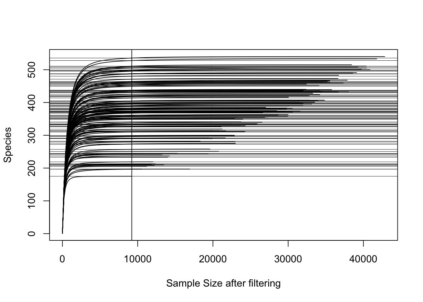
Check if you cover enough depth for diversity analyses. In this case I had to remove references, blanks, autoclaved soils and soils treated with hydrogen peroxide before doing diversity analyses.
#filter
`%notin%` = Negate(`%in%`)
#physeqB.flt.norefs <-  prune_samples(sample_data(physeqB.flt)$Name %notin% c("41AutoclavedControlT0","42AutoclavedControlT0","43AutoclavedControlT0","44AutoclavedControlT0"), physeqB.flt)
physeqB.flt.norefs <-  prune_samples(sample_data(physeqB.flt)$Treatment %notin% c("Heat", "H2O2"), physeqB.flt)
physeqB.flt.norefs <-  prune_samples(sample_data(physeqB.flt.norefs)$Treatment != "Reference", physeqB.flt.norefs)
physeqB.flt.norefs <-  prune_samples(sample_data(physeqB.flt.norefs)$Treatment != "Blank", physeqB.flt.norefs)
physeqB.flt.norefs <-  phyloseq::prune_taxa(taxa_sums(physeqB.flt.norefs) != 0, physeqB.flt.norefs)

vegan::rarecurve(t(otu_table(physeqB.flt.norefs)), step=200, sample = min(colSums(otu_table(physeqB.flt.norefs))), label = FALSE, xlab = "Sample Size after filtering")

Prevelance table
Create a prevalence table to see which phyla have low prevalence
## Create a prevalence table to see which phyla have low prevalence
physeqB.flt.prevtab <-  prune_samples(sample_data(physeqB.flt)$Treatment != "Reference", physeqB.flt)
physeqB.flt.prevtab <-  prune_samples(sample_data(physeqB.flt.prevtab)$Treatment != "Blank", physeqB.flt.prevtab)
prevelancedf = apply(X = phyloseq::otu_table(physeqB.flt.prevtab),
                       MARGIN = 1,
                       FUN = function(x){sum(x > 0)})
prevelancedf = data.frame(Prevalence = prevelancedf,
                            TotalAbundance = taxa_sums(physeqB.flt.prevtab),
                            phyloseq::tax_table(physeqB.flt.prevtab))

prevelancedf <- plyr::ddply(prevelancedf, "Phylum", function(df1){
  data.frame(mean_prevalence=mean(df1$Prevalence), total_abundance=sum(df1$TotalAbundance,na.rm = T), stringsAsFactors = F)
  })
prevelancedf
##               Phylum mean_prevalence total_abundance
## 1    Acidobacteriota        7.214912          199741
## 2   Actinobacteriota        8.756279          708045
## 3     Armatimonadota        4.954545            2062
## 4       Bacteroidota        5.981818           20919
## 5   Bdellovibrionota        3.000000              30
## 6        Chloroflexi        9.567042          646439
## 7      Cyanobacteria        3.333333             135
## 8       Dependentiae        3.333333              72
## 9   Desulfobacterota        4.875000            1572
## 10        Firmicutes       14.844250         1101043
## 11   Gemmatimonadota        5.800000           17851
## 12       Myxococcota        5.909091           27926
## 13      Nitrospirota        4.235294            2300
## 14   Planctomycetota        6.509174          177762
## 15    Proteobacteria        8.713961          557906
## 16           RCP2-54        6.666667            3067
## 17 Verrucomicrobiota        8.205128           54178
## 18             WPS-2        5.870968           20024
Note:
This code is an amalgamation from various sources. Apart from putting it together into a pipeline I do not take credit for it.